Paper URL: http://proceedings.mlr.press/v139/trauble21a/trauble21a.pdf
What?
- Authors study the performance of 6 popular disentanglement methods across 5 datastets in which two ground truth factors have (synthetically generated) pariwise linear correlation.
- They also propose two methods to resolve the entanglement of latent dimensions caused by correlation. First method requires additional labels to be available for correlated factors, whereas the second method only needs pairs of observations which differ in an unknown number of factors – but no labels.
Why ?
The datasets used to learn and demostrate disentanglement use completely independent FoVs with factorized joint distribution i.e. p(\textbf{c}) =\prod_{i=1}^n p(c_i) and the methods themselves use factorized priors p(\textbf{z}) =\prod_{i=1}^n p(z_i) to represent these FoVs. This independence assumption won’t hold in real world where (groups of) factors might exhibit correlation due to direct causation or confounding. Thus it is important to know how current methods behave in that setting.
Additionally:
- Learning correlations between sensitive attributes like race, sex etc. and has implications for fairness of representation.
- Correlated latents won’t allow interventions independent of other variables, thus limiting our ability to interpret and inspect models.
How?
How do disentanglement methods perform on correlated data?
Their emperical study with ~4000 models shows the following trends:
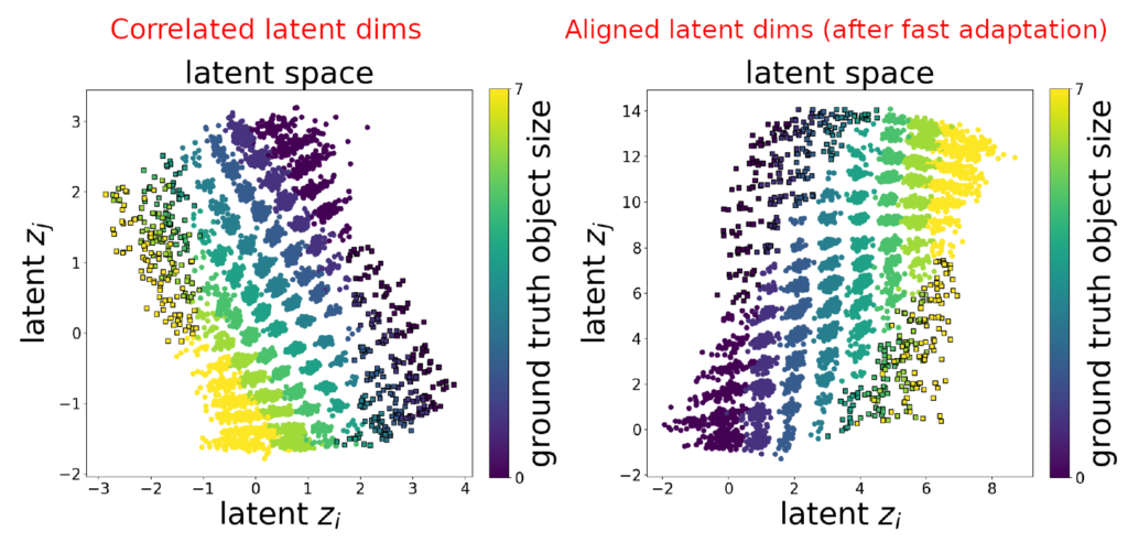
- Models encode the two correlated FoVs simultaneously with two latent units i.e. changing value of either latent unit will affect two factors of generative process. When this happens, one unit usually captures correlation across major correlation axis whereas the other unit captures correlation across minor axis.
- Models can still disentangle FoVs if (linear pairwise) correlation is low, but the performance degrades with stronger correlation.
- Models can construct meaningful images for latent combinations it has never seen before i.e. zero probability under generative model. The latent space encodings of such OOD examples are also meaningful and exhibit extrapolation generalization. This is in contrast to negative results (in case of uncorrelated datasets) for combinatorial interpolation generalization.
Crucially: if some FoVs are correlated in the dataset, generative model that matches the true likelihood p^∗(x) cannot be disentangled. In that case, ELBO optimization has a bias against disentanglement. Consider for \textbf{z} \in \mathbb{R}^3 , if we have independent prior in our generative model p(\textbf{z}) = p(z_1)p(z_2)p(z_3) versus the true latent distribution (with correlation) p(\textbf{z}) = p(z_1)p(z_2)p(z_3|z_2) . In this case, the learned latent distribution q(\textbf{z}|\textbf{x}) will have lower likelihood value if it is not factorized because of KL divergence KL(q(\textbf{z}|\textbf{x})||p(\textbf{z})) with an independent prior in the ELBO objective.
How to resolve latent correlations ?
Method 1: When some labels are available (fast adaptation)
Authors provide a supervised procedure that can disentagnle correlated latents given only very few labels related to the correlated factors. First, identify entangled latent pair of units (z_i,z_j) by looking at feature importances of GBTs. Intuitively, if correlated factors (c_1,c_2) are encoded by two latents z_{i} and z_j then they will have relatively high feature importance w.r.t both c_1 and c_2. Then, train a substitution function f_\theta : \mathbb{R}^2 \rightarrow \{0,...,c_{max}^1\} \times \{0,...,c_{max}^2\} using the given labels to infer values of FoVs from z_{i} and z_j. Then use this prediction f_\theta(z_{i},z_j) = (c_1,c_2) to replace the values of entangled dimensions. Limitations of this have been discussed in Appendix D.
Method 2: When no labels are available (Ada-GVAE with k=1)
Use Ada-GVAE (weakly-supervised) approach which needs a pair of observations (\textbf{x}^1,\textbf{x}^2) that differ in an unknown number of factors. It infers common factors via dimension-wise KL divergence: KL(q(\textbf{z}|\textbf{x}^1)||q(\textbf{z}|\textbf{x}^2)) . Intuitively, dims corresponding to common factors will have a lower KL divergence. Once we have such pairs, we re-train the network over these examples with a modified \beta-VAE objective. In the paper they only consider pairs which differ in 1 factor.
Be First to Comment