What?
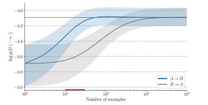
Authors tackle the question of how the direction of causality i.e. A \rightarrow B or B \rightarrow A can be inferred from rate of adaptation of model. Intuitively speaking model trained according to correct causal graph will need to update only a few of its parameters and hence should converge faster.
Why?
Inferring direction of causality in bivariate case is notoriously difficult because of absence of conditional indepencies. They make a fairly common assumption that if the true generative process consists of independent causal mechanisms that don’t interfere with each other like P(A) and P(B|A) then interventions can be assumed to be localized to one or few modules e.g to P(A). This would then translate to needing to only adapt the parameters associated with that specific module.
They also use a smooth parameterization of the considered causal graph to directly optimize this score in an end-to-end gradient-based manner.
How?
Train on a dataset \mathcal{D_{obs}} to get \hat{\theta}_G^{ML}(\mathcal{D_{obs}}) , then assume that we get some new samples from interventional / transfer distribution \mathcal{D_{int}} \sim \tilde{p} i.e. we intervene on the cause X which changes (only) p(X) to \tilde{p}(X) . Then optimize the loss over new dataset as follows:
\mathcal{L}_G(\mathcal{D_{int}}) = \prod_{t=1}^T p(x_t; \theta_G^{(t)}, G)
\\[8pt]
\theta_G^{(1)} = \hat{\theta}_G^{ML}(\mathcal{D_{obs}})
\\[8pt]
\theta_G^{(t + 1)} = \theta_G^{(t)} + \alpha \nabla_{\theta} \log p(x_t; \theta_G^{(t)}, G)
\\[8pt]
\mathcal{R}(\mathcal{D}_{int}) = -\log[\sigma(\gamma) \mathcal{L}_{A \rightarrow B}(\mathcal{D}_{int}) + (1-\sigma(\gamma))\mathcal{L}_{B \rightarrow A}(\mathcal{D}_{int})]
Here we represent our belief that p(A \rightarrow B) = \sigma(\gamma) (respectively, p(B \rightarrow A) = 1 - \sigma(\gamma) ), with \gamma learned from data.
And?
- They provide details on how the approach could be generalized to n variables by representing the graph via an n \times n adjacency matrix B with degree of belief about pair-wise causal direction between vertices V_i and V_j i.e. B_{ij} sampled from a Bernoulli. The idea is then to learn these parameters from data.
- The idea makes intuitive sense and is also supported by previous work which explores the same problem but used formalism of Kolmogorov complexity and Minimum Description Length e.g. see A. Marx and J. Vreeken’s SLOPPY .
- I wonder how the method would fare when (1) the fitted model class is different (2) model capacities are different. Would it have enought “resolving power” to still distinguish the correct directions? I think that we’d lose resolving power as model grows complex enough that we could have trade-off between (some) wrong causal directions.
Be First to Comment